Motivation
Catch your breath, because the Poisson distribution isn’t as complicated as it looks. You’ve probably seen this intimidating formula before:
\[P(\text{$k$ events occur})=\frac{\lambda^k}{k!}e^{-\lambda}\]
Most of us end up memorizing it, hoping it makes sense someday. But this isn’t because the Poisson is particularly hard; it’s because the Poisson is introduced early on in probability theory — long before we have the mathematical tools to really understand it.
My mission is to demystify the Poisson and offer an intuitive way to remember it. I’ll break down each term, giving you a clear and satisfying understanding right from the beginning of your probability journey.
What is the Poisson?
Suppose we have a timeline showing a single time period.

The Poisson deals with the number of “events” that occur in the time period. Each time an event occurs, we’ll place a point at the time it happens.

Think about the number of events we could have: we could have \(0\) events, \(1\) event, \(2\) events, or any number \(k\) events.
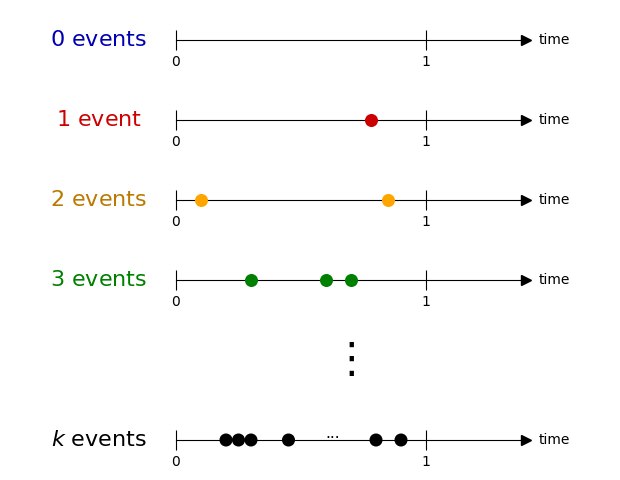
The Poisson’s only parameter \(\lambda\) is the average number of events, meaning on average we see \(\lambda\) events:

\(\lambda\) is known as the event rate, and it can take on many forms:
| How many customer service calls does a call center expect to receive in an hour? | \(\lambda=\text{calls/hour}\) |
| How many cars do I expect to pass in front of a billboard in a day? | \(\lambda=\text{cars/day}\) |
| How many patients will arrive at an emergency room in an hour? | \(\lambda=\text{patients/hour}\) |
Can we use \(\lambda\) to derive the entire distribution? Of course!
What’s a Measure?
Suppose I randomly throw darts at a dartboard, and I want to know the probability I hit the bullseye.
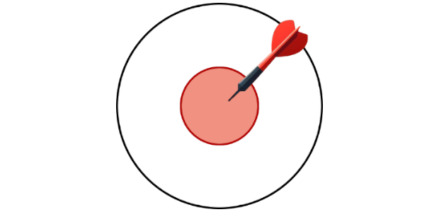
Loosely speaking, every point within the bullseye is a unique way we could hit the bullseye, and every point on the board is a unique way we could hit the board. We can take the ratio of these “number of ways” to find the probability:
\[P({\color{#b51313} {\text{I hit bullseye}} })=\frac{\color{#b51313} {\text{number of ways of “hitting a bullseye”}}}{\color{#000000} {\text{number of ways of “hitting anywhere on the board”}}}\]
More specifically, we can measure these “number of ways” by the size of the bullseye and the size of the entire board.
\[P({\color{#b51313} {\text{I hit bullseye}}})=\frac{\color{#b51313} {\text{size of “hitting a bullseye”}}}{\color{#000000} {\text{size of “hitting anywhere on the board”}}}\]
Pretty intuitive, right? We’ll do something similar for the Poisson — we just have to figure out how to measure things.
Measuring the Poisson
We can set the Poisson distribution up just like the dartboard example:
\[P({\color{#b51313} {k \text{ events happen}}}) = \frac{\color{#b51313} {\text{size of “$k$ events happening”}}}{\color{#000000} {\text{size of “any number of events happening”}}}\]
How many ways can 0 events happen?
We’ll start with the easiest case, there are no events in the interval. How many “ways” can no event happen?

Just \(1\). The picture I drew above is the only picture I could have drawn showing \(0\) events in the interval. No event occurs at every possible point in time.
So the “number of ways” in which \(0\) events can happen is \(\color{#1b1b9f} {1}\).
How many ways can 1 event happen?
Consider a few individual cases in which \(1\) event happens:

Each of these corresponds to a “possible time” in which a single event could occur. If we plot each case on a single timeline, you’ll see that each case is just an individual point in the interval:

If we plot every possible point, we’d just get the interval itself. In other words, all the points in which a single event could occur are contained within the interval:

So the “number of ways” in which a single event could occur is just the size of the interval:

We can measure the interval however we want, so long as we measure all intervals in a consistent way. In this case, we’ll use the “average number of events” that occur within the interval as our notion of “size”. That means the interval has a length of \(\lambda\):

Therefore the “number of ways” in which \(1\) event can happen is \(\color{#CC0000} {\lambda}\)
How many ways can 2 events happen?
As before, we’ll consider a few individual cases involving \(2\) events:

We can visualize these cases at the same time by adding an extra time axis to our earlier plot. The x-axis will be the time at which the first event occurs, and the y-axis will be the time at which the second event occurs.

Then points within this 2-dimensional space correspond to unique combinations of 2 events.
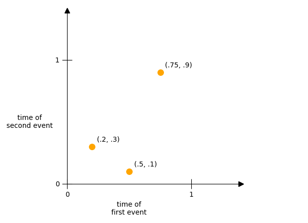
If we plot every possible point, we’d just get the area itself. In other words, all the points in which two events could occur are contained within the area.
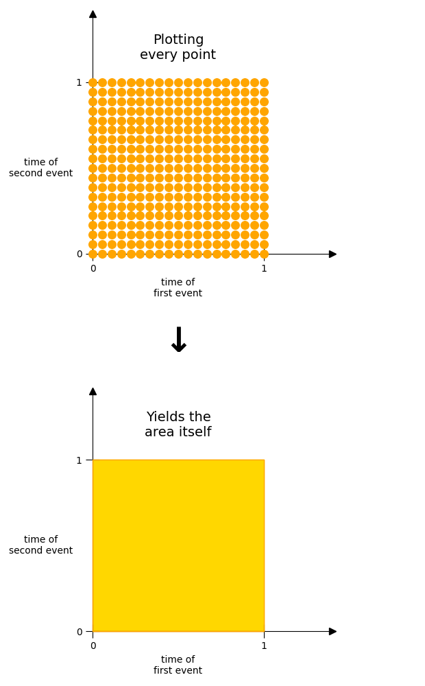
And what’s more, it’s very easy to measure the size of this. We know that each individual interval has a length of \(\lambda\)

So this new area must have a size of \(\lambda^2\)
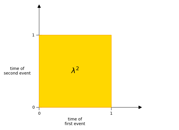
Well this is almost right; we’re actually over-counting things. This is because we don’t want to distinguish between the order of events.
Consider the case in which one event happens at \(.2\) and another at \(.8\):

Our current approach is counting this case twice. There are \(2\) ways this could happen, and our current approach is counting both of them:

Therefore the point \((.2, .8)\) is equivalent to the point \((.8, .2)\).
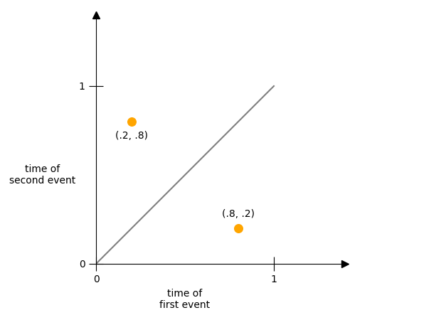
We’ve over-counted by the number of ways \(2\) events can be arranged — that is, by a factor of \(2\). Let’s show this graphically.
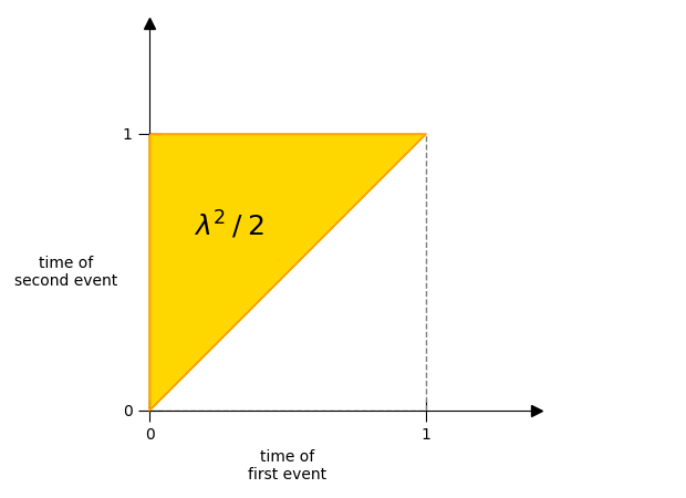
Putting everything together, the “number of ways” in which \(2\) events can occur is \(\color{#ba7900} {\lambda^2 / 2}\)
How many ways can 3 events happen?
As before, we’ll add an extra time axis to our last plot. The x-axis will be the time at which the first event occurs, the y-axis will be the time at which the second event occurs, and the z-axis will be the time at which the third event occurs:
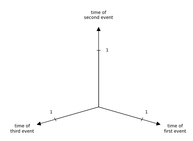
And just like before, we also know how to measure this. We know that each interval has a length of \(\lambda\)
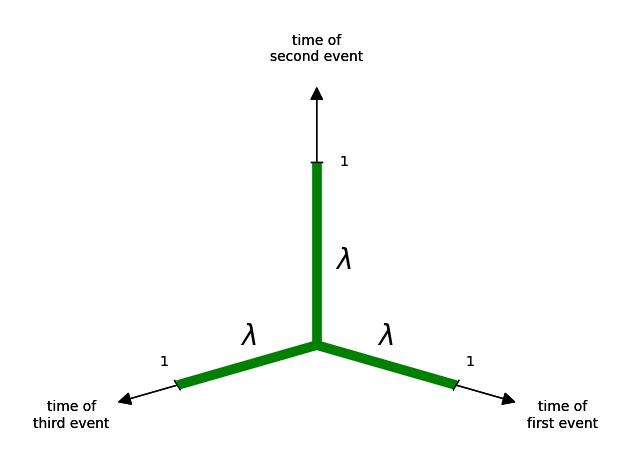
So the entire volume must be \(\lambda^3\)
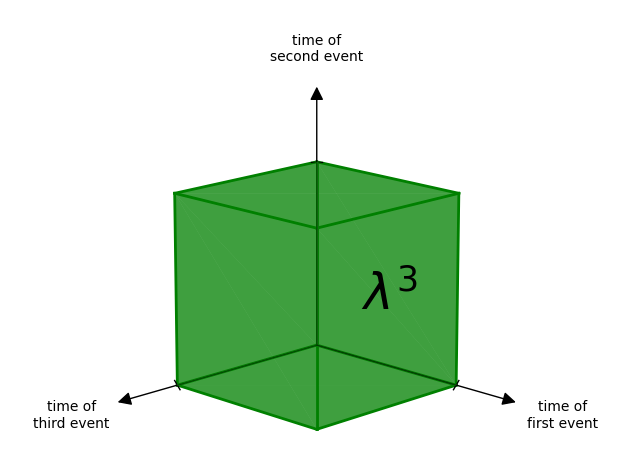
But since we don’t care about the order of events, we’ve overcounted again.
Consider the case in which one event happens at time \(.1\), another at time \(.5\), and one more at time \(.9\):

Our current approach is counting this one case \(6\) times. That’s because there are \(3!=6\) different ways the events can be arranged, and our approach is counting all of them:
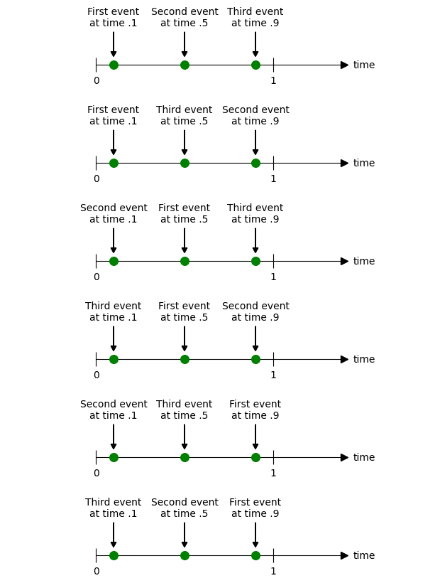
Therefore the following points are equivalent to one another:
- \((.1, .5, .9)\)
- \((.1, .9, .5)\)
- \((.5, .1, .9)\)
- \((.5, .9, .1)\)
- \((.9, .1, .5)\)
- \((.9, .5, .1)\)
We can visualize these points as follows:
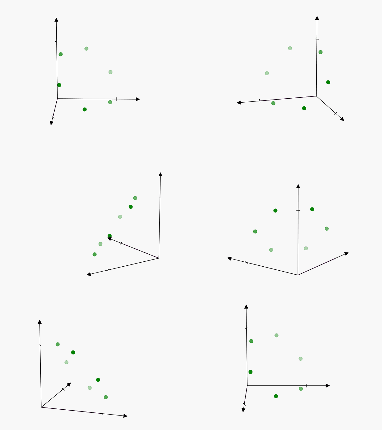
The axes of symmetry are harder to visualize in 3-dimensions than in the previous 2-dimensional example, but the concept is the same. Each of these points represents the same thing:
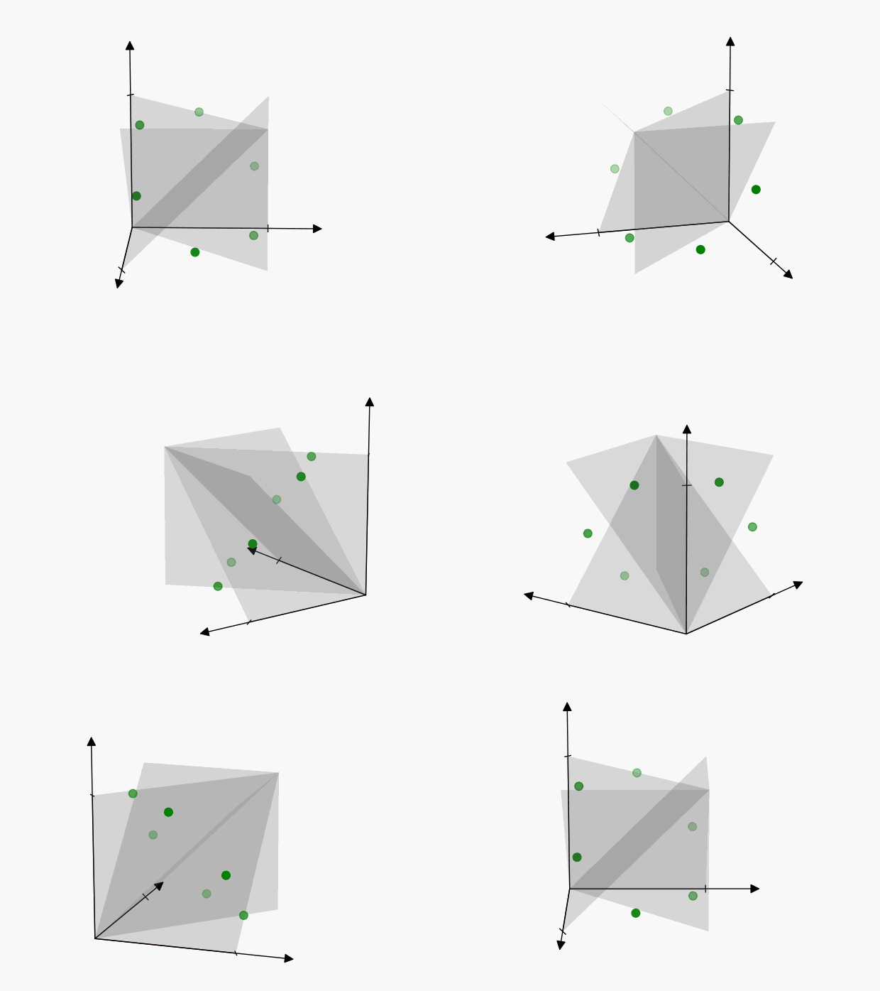
To account for this, we’ll have to reduce the volume of our cube by \(3!\), so that we only include one of the points:
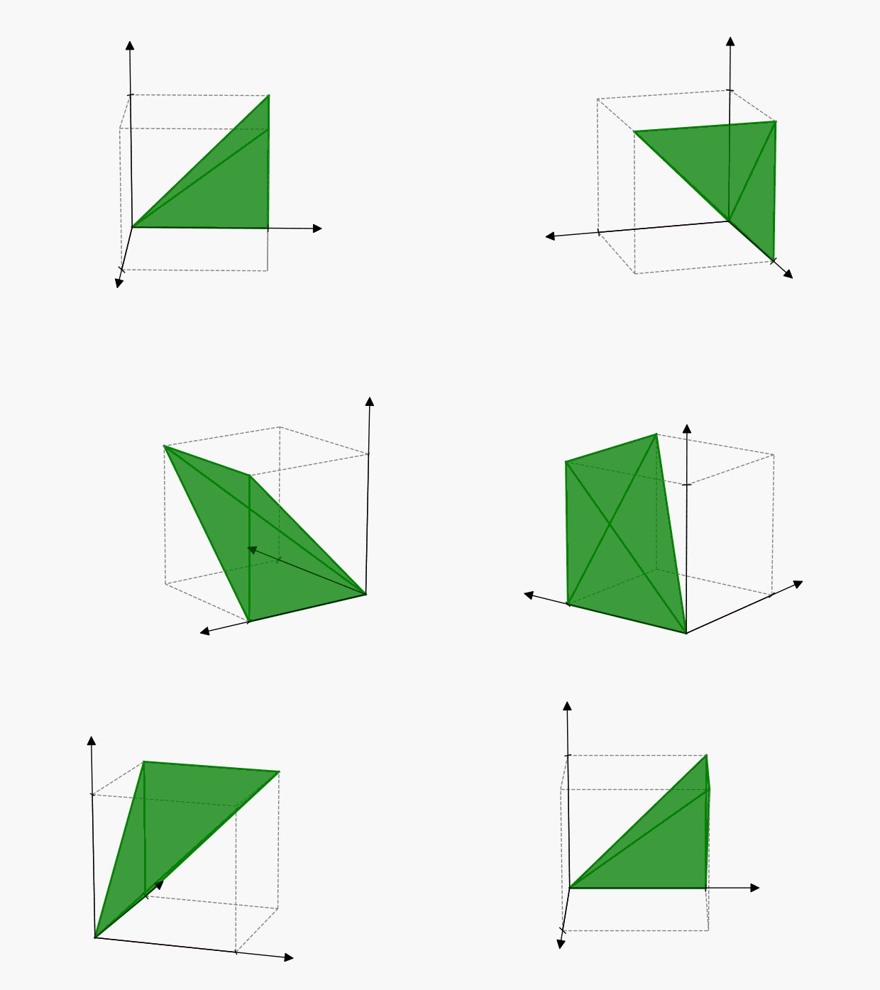
Therefore the “number of ways” in which \(3\) events can happen is \(\color{green} {\lambda^3 / 3!}\)
Note that it’s not actually important to be able to visualize this shape exactly. What’s important is the pattern. I’m only visualizing the shape here, so the pattern feels more concrete.
How many ways can k events happen?
Now we can extend the pattern for any \(k\) successes. We can’t visualize more than 3-dimensions, but the same pattern holds.
We’ll add a time axis for each additional event, which will multiply our volume by \(\lambda\). When we do this \(k\) times, the resulting volume will be \(\lambda^k\)
But as before, we’ll be over-counting by the number of ways we can arrange \(k\) events, so we’ll reduce our volume by \(k!\)
Therefore the “number of ways” in which \(k\) events can happen is \(\color{#b51313} {\lambda^k/k!}\)
And finally! We’ve made sense of one of the terms in the Poisson.
\[P({\color{#b51313} {\text{$k$ events happen}}})={\color{#b51313} {\frac{\lambda^{k}}{k!}}} e^{-\lambda} \]
Measuring the Sample Space
The sample space is the case in which any number of events could happen. Recall from earlier the number of possible events: we could have \(0\) events, \(1\) event, \(2\) events, \(3\) events, \(\dots\)
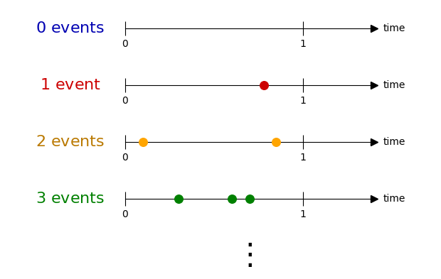
The size of the sample space is just the size of all these added together.
\[\text{size of sample space}\]
\[= \color{#1b1b9f} {\text{ size of “0 events happening”}}\]
\[+ \color{#CC0000} {\text{ size of “1 event happening”}}\]
\[+ \color{#ba7900} {\text{ size of “2 events happening”}}\]
\[+ \color{green} {\text{ size of “3 events happening”}}\]
\[+ \dots\]
We already know how to measure these. Let’s use our \(\lambda^k/k!\) formula to measure every case:
| Size of \(0\) events happening | \(\color{#1b1b9f} 1\) |
| Size of \(1\) event happening | \(\color{#CC0000} \lambda\) |
| Size of \(2\) events happening | \(\color{#ba7900} {\lambda^2 / 2}\) |
| Size of \(3\) events happening | \(\color{green} {\lambda^3 / 3!}\) |
| … | \(\dots\) |
\[\text{size of sample space}= {\color{#1b1b9f} {1}} + {\color{#CC0000} {\lambda}} + {\color{#ba7900} {\lambda^2/2}} + {\color{green} {\lambda^3/3!}} + \dots = \sum_{k=0}^{\infty} \lambda^k/k!\]
Those of you familiar with \(e\) should recognize that
\[\sum_{k=0}^{\infty} \lambda^k/k! = \color{#000000} {e^\lambda}\]
Or expressed graphically:

So \(e^\lambda\) is just the size of the sample space! We’ve now made sense of the final term in the Poisson PMF:
\[P(\text{$k$ events happen})= {\frac{\lambda^{k}}{k!}} \color{#b51313} {{e^{-\lambda}}}\]
If you’re a little rusty on your \(e\) definitions, I’d look at the excellent \(e\) articles by Better Explained:
Putting things together
Now that we know what all the terms mean, the formula for the Poisson PMF becomes very straightforward.
\[P({\color{#b51313} {\text{$k$ events happen}}})=\frac{{\color{#b51313}{\text{size of “$k$ events happening”}}}}{{\color{#000000}{\text{size of sample space}}}}\]
\[P({\color{#b51313} {\text{$k$ events happen}}})=\frac{\color{#b51313} {\lambda^k/k!}}{\color{#000000} {e^\lambda}}\]
Or how it’s usually written:
\[P({\color{#b51313} {\text{$k$ events happen}}})={\color{#b51313} {\frac{\lambda^k}{k!}}} {\color{#000000} {e^{-\lambda}}}\]
See? That formula isn’t so scary.

Leave a Reply